The guide below has been prepared to help HPC users effectively utilize our system. This is a quick guide; for a detailed explanation, please visit our BeoShock Wiki Page.
Supporting Documents
Please refer to our Beoshock Wiki page for a comprehensive guide on using the HPC system.
Access and Login
Click the '+' to expand each section.
All WSU constituents and outside of WSU who are KBOR constituents are eligible for the BeoShock account. To request an HPC user account, go to New User Request, press ‘New HPC Access’ button and fill in/select appropriate items. The approval for the account will be granted in few business days.
Once the access is granted, you can use your myWSU credentials to log on to the cluster using ssh from a terminal. You will automatically be enrolled in the listserv HPC-USERS-L@listserv.wichita.edu for current, ongoing HPC user information. Do not unsubscribe from this listserv because it will result in your HPC account being closed. From time to time there is maintenance on the HPC system and this will be the primary mechanism to communicate to all HPC users.
An SSH (Secure Shell) client is required to connect to BeoShock. SSH is usually available on Linux and macOS machines, and you need to open a terminal and use your WSU credential to login
ssh wsu_id@hpc-login.wichita.edu
The WSU ID should be in lower case.
There are many SSH clients for Windows, such as PuTTY and MobaXterm. Download and install the SSH client for Windows machines. Open the SSH client and start a terminal to log in using the WSU credential. Here is the more detailed video tutorial for installing and using SSH client: Video 1: "How to Log In"
Graphical Interface for Connecting to BeoShock via Web Browser
Open OnDemand is a web-based graphical interface designed to simplify access and use of High-Performance Computing resources. It allows users to connect to the BeoShock HPC cluster directly from a web browser without the need for complex command-line tools or additional software installations.
How Does It Make HPC Easier?
- User-Friendly Interface: Open OnDemand provides an intuitive dashboard where users can upload and download files, monitor job status, and submit jobs using graphical tools.
- Remote Access: Users can access HPC resources from anywhere through a secure web connection, removing the need for on-site access.
- Interactive Sessions: Users can launch interactive sessions, such as Jupyter notebooks or graphical desktop environments, to visualize and analyze data directly.
Open a web browser such as Firefox (if off-campus, use the VPN first) and go to: ondemand.hpc.wichita.edu
Then you will be prompted for your username and password, use the same credentials (username should be all lower cases) you use to access the login node for the BeoShock.

To have the best experience using the Open OnDemand, please use the latest versions of Google Chrome, Mozilla Firefox or Microsoft Edge. Use any modern browser that supports ECMAScript 2016. The Open Ondemand does not support IE. Safari is partially supported and may cause problems when using the Open OnDemand.
Open OnDemand, developed by the Ohio Supercomputer Center, is supported by funding from the National Science Foundation. To learn more about the Open OnDemand project, please visit their official website.
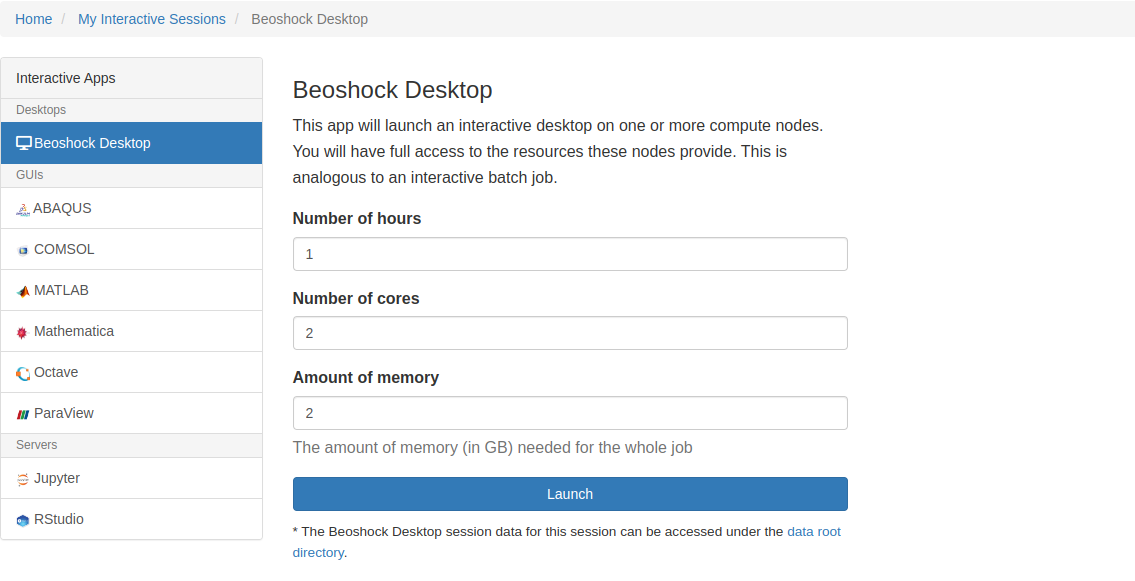
Some interactive apps are supported from the Open OnDemand portal: BeoShock Desktop, Octave, Jupyter, Mathematica, RStudio, and ParaView. These applications can be accessed by selecting "Interactive Apps" from the home page. You can choose the number of hours, number of cores, and amount of memory when launching these applications. If you finish early, return to the “My Interactive Sessions” tab and delete the job.
VPN for HPC Users
Secure Remote Access with VPN
All HPC users are automatically provisioned with access to BeoShock HPC upon installing the VPN. If you are off-campus, you must configure and use the Virtual Private Network (VPN) to securely connect to HPC resources.
For setup instructions and additional details:
1. Visit the VPN Information Page for guidance.
2. Follow the instructions on the page to install and configure the VPN.
For further assistance, contact the ITS Helpdesk
Open Support Session
Transferring Data
SCP (secure copy) is a command-line utility uses ssh for securly data transfer between two locations. It requires an password to authenticate on the BeoShock. For example, copy a file from a local system to BeoShock:
scp myfile wsu_id@hpc-login.wichita.edu:/your/directory
To copy a local directory to BeoShock:
scp -r my_directory wsu_id@hpc-login.wichita.edu:/your/directory
SFTP (SSH File Transfer Protocol) is a secure file protocol to transfer and manage files betweem two locations. Similar to the SCP, SFTP performs all operations over an encrypted ssh session. For example, put file from local system to BeoShock:
sftp wsu_id@hpc-login.wichita.edu
put myfile
put -r my_directory
On the Open OnDemand home page, select left most "Files", it will bring up a file manager interface. By default, it will show files in your home directory. You can do file operations by selecting the file in the main window panel and selecting the desired operation from the main menu as marked. If you want to edit the file, select the file you wish to edit, and select "Edit" from the main menu. This will open up a text editor in a new tab. You can also click the "Upload" button to open a dialog that will allow you to navigate your local computer and select which files you want to upload. To download files, you must select the file you wish to download, and then click the "Download" button.

To use the Globus web application, you can go to https://www.globus.org/ and click on "Log In" in the upper right corner of the page. Type or find the "Wichita State University" in the Organization box and click continue. You will need the WSU credentials to log in.

After logging in with your WSU credentials, you should reach the data transfer page. Turn on the two-panel mode by clicking the switch on the top right. On this page you will get two file browser windows, each window represents the two systems you wish to transfer files. In the "Collection Search" on the left, type "BeoShock Filesystem," then it will show files in your home directory on BeoShock. If you want to transfer files through other endpoints (i.e., other HPC or research institutions), search the endpoint at right. Then you can navigate to the path in your file tree and select the file you wish to transfer. Next, press "Start" to initiate the transfer of files.

Environment Modules
Many commonly used software has been built on the BeoShock and can be used as environment modules. To get a list of the installed modules:
module avail
The output of "module avail" can be quite long, so you can narrow the list down by specifying a string, e.g.
module avail python
To see information about a module, you can use:
module show module_name
You can list which modules have been loaded:
module list
You can then load a module:
module load module_name
If you want to unload a module:
module unload module_name
or to unload all loaded modules:
module purge
Basic Job Submission
Slurm is an open source cluster management and job scheduling system that allow users to run their jobs on Boeshock. The user can specify the allocated resources for scheduling the job through the script. You create and edit a script using a text editor of your choice, such as nano, vim, emacs, or any other text editor available in the HPC system. Here is a simple job submission script:
#!/bin/bash

#Submit this script with: sbatch my_slurm.sh

#SBATCH --job-name=test
#SBATCH --time=1:00:00   # time
#SBATCH --ntasks=1   # number of processor cores (i.e. tasks)
#SBATCH --nodes=1   # number of nodes
#SBATCH --mem-per-cpu=1G   # memory per CPU core

# Load module
  module load #your_software

# Navigate to the directory where the executable/script is located
  cd /path/to/directory_containing_run_executable

# Execute the script
To submit the job to the cluster, use:
sbatch my_slurm.sh
For more information, please refer to Slurm Documentation
In a job script, lines begin with #SBATCH in all caps is treated as a Slurm command. When you want to comment out a Slurm command, you need to append a second another pound sign # to the #SBATCH, i.e., ##SBATCH. Here is a list of SBATCH options.
SBATCH --job-name=<name>: gives the name to the job.
SBATCH --output=<name>: the output file.
SBATCH --partition=<name>: the specific partition of the resource allocation.
SBATCH --ntasks-per-node=<number>: number of tasks per node.
SBATCH --cpus-per-task=<number>: number of CPUs per task.
SBATCH --mem-per-cpu=<memory>: set the minimum memory required per CPU.
SBATCH --time Days-Hours:Minutes:Seconds: set the time limit for the job.
SBATCH --mail-user=<email>: email address for the notifications of job status.
SBATCH --mail-type=<type>: BEGIN for when job starts, END for when the job ends, FAIL for when the job fails, ALL for all circumstances.
#SBATCH --gres=gpu: <ngpus>: specify number of GPUs needed for your job.
The Slurm job controller will pass the information (i.e., working directory, number of CPUs, etc.) contained in the batch script to a scheduled job via environment variables. The following is a list of commonly used informational environment variables.
$SLURM_JOB_ID: the job ID.
$SLURM_SUBMIT_DIR: the directory you were in when submit jobs.
$SLURM_CPUS_ON_NODE: how many CPUs were allocated on this node.
$SLURM_JOB_NAME: the job name.
$SLURM_JOB_NODELIST: the list of nodes assigned to job.
$SLURM__CPUS_PER_TASK: number of CPUs per task.
$SLURM_MEM_PER_CPU: memory per CPU.
$SLURM_MEM_PER_GPU: memory per GPU.
$SLURM_NTASKS: the number of tasks.
A full list of environment variables for Slurm can be found at Slurm Environment Variables
To request GPU resources, add the line with "--gres=gpu:count" to the job script. Here is an example:
#!/bin/bash
#Submit this script with: sbatch thefilename
#SBATCH --job-name=test#SBATCH --time=1:00:00 # time
#SBATCH --ntasks=1 # number of processor cores (i.e. tasks)
#SBATCH --nodes=1 # number of nodes
#SBATCH --mem-per-cpu=1G # memory per CPU core
#SBATCH --gres=gpu:1 # request 1 gpu
# LOAD MODULES, INSERT CODE, AND RUN YOUR PROGRAMS HERE
python example.py #run python script
You can run an interactive job using the "srun" command. The following command requires a single core and default amount of memory for one hour:
srun --nodes=1 --ntasks-per-node=1 --time=01:00:00 --pty bash -i
When you are done with interactive jobs, use "exit" to get back to headnode mode.
You can check the status of all your running jobs:
squeue -u wsuid
You can delete your job by specifying the job id:
scancel JOBID
Python
BeoShock has Python 2 and Python 3 modules available. To check the available Python module:
module avail Python
To load the Python module:
module load Python/version_you_want
Below is the sample Slurm script (python.slurm),
#!/bin/bash
#SBATCH --job-name=py-job        # create a short name for your job
#SBATCH --nodes=1                # node count
#SBATCH --ntasks=1               # total number of tasks across all nodes
#SBATCH --cpus-per-task=1        # cpu-cores per task (>1 if multi-threaded tasks)
#SBATCH --mem-per-cpu=4G         # memory per cpu-core (4G per cpu-core is default)
#SBATCH --time=00:01:00          # total run time limit (HH:MM:SS)


module purge
module load Python/3.9.6-GCCcore-11.2.0

python myscript.py
Then your python job can be submitted to the cluster:
sbatch python.slurm
For more information about Python documentation, check https://www.python.org/.
To install the python packages, you will need to create the virtual enviroment, try the following procedure to install your package(s).
First, load a Python module:
module load python/version_you_want
Next, create the location of virtual Python environment in your home directory and then create a virtual environment:
mkdir /path/to/virtualenvs
cd /path/to/virtualenvs
virtualenv test
We have created a virtual environment called "test". Then, activate the virtual environment:
source /path/to/virtualenvs/test/bin/activate
Now you can install the python packages, for example, install "mpi4py" by
pip install mpi4py
In this section, let's create a Python3 script named hello_world.py.
#!/usr/bin/env python3
# -*- coding: utf-8 -*-#Hello world example
from mpi4py import MPI
comm = MPI.COMM_WORLD #get the information about all the processors run script
name = MPI.Get_processor_name() #get the processor's name
rank = comm.Get_rank() #gives identifier of the processor which currently executing the code
size = comm.Get_size() #gives the total number of ranks
print("Hello world from node", str(name), "rank", rank, "of", size)
Load the module of Python3 and the virtual environment in which you install the "mpi4py", and then you can run the script with:
mpiexec -n 5 python hello_world.py # run 5 processes
The output will be similar to the following:
Hello world from node headnode01.beoshock.wichita.edu rank 0 of 5
Hello world from node headnode01.beoshock.wichita.edu rank 3 of 5
Hello world from node headnode01.beoshock.wichita.edu rank 4 of 5
Hello world from node headnode01.beoshock.wichita.edu rank 1 of 5
Hello world from node headnode01.beoshock.wichita.edu rank 2 of 5
If you try this example, the output may not be in the same order as shown above. This is because 5 separate processes are running on different processors, and we cannot know which one will execute its print statement first.
Here is a simple job script using MPI with Python:
#!/bin/bash
#SBATCH --ntasks=8
#SBATCH -t 00:00:30
#SBATCH --nodes=4
module load Python/version_you_want
module load OpenMPI/some_verison
source /path/to/virtualenvs/test/bin/activate
export PYTHONDONTWRITEBYTECODE=1
mpirun python /path/to/hello_world.py
Toolchains
A toolchain is a set of compilers, libraries, and applications that are needed to build software. Some software functions better when using specific toolchains. We provide a good number of toolchains and versions of toolchains to make sure your applications will compile and/or run correctly. These toolchains include (you can run 'module keyword toolchain'):
foss: GNU Compiler Collection (GCC) based compiler toolchain, including OpenMPI for MPI support, OpenBLAS (BLAS and LAPACK support), FFTW and ScaLAPACK.
fosscuda: GCC based compiler toolchain __with CUDA support__, and including OpenMPI for MPI support, OpenBLAS (BLAS and LAPACK support), FFTW and ScaLAPACK.
gompi: GNU Compiler Collection (GCC) based compiler toolchain, including OpenMPI for MPI support.
gompic: GNU Compiler Collection (GCC) based compiler toolchain along with CUDA toolkit, including OpenMPI for MPI support with CUDA features enabled.
intel: Intel Compiler Suite, providing Intel C/C++ and Fortran compilers, Intel MKL & Intel MPI. Recently made free by Intel, we have less experience with Intel MPI than OpenMPI.
iomkl: Intel Compiler Suite, providing Intel C/C++ and Fortran compilers, Intel MKL & OpenMPI. Recently made free by Intel, we have more experience with OpenMPI than Intel MPI.
gcccuda: GNU Compiler Collection (GCC) based compiler toolchain, along with CUDA toolkit.
Tk: Tk is an open source, cross-platform widget toolchain that provides a library of
basic elements for building a graphical user interface (GUI) in many different programming
languages.
You can run 'module spider toolchain/' to see the versions we have:
module spider fosscuda
If you load one of the fosscuda (module load fosscuda/2020b), you can see the other modules and versions of software been loaded with "module list":
Currently Loaded Modules:
1) GCCcore/10.2.0 9) XZ/5.2.5-GCCcore-10.2.0 17) libfabric/1.11.0-GCCcore-10.2.0
2) zlib/1.2.11-GCCcore-10.2.0 10) libxml2/2.9.10-GCCcore-10.2.0 18) PMIx/3.1.5-GCCcore-10.2.03) binutils/2.35-GCCcore-10.2.0 11) libpciaccess/0.16-GCCcore-10.2.0 19) OpenMPI/4.0.5-gcccuda-2020b
4) GCC/10.2.0 12) hwloc/2.2.0-GCCcore-10.2.0 20) OpenBLAS/0.3.12-GCC-10.2.0
5) CUDAcore/11.1.1 13) libevent/2.1.12-GCCcore-10.2.0 21) gompic/2020b
6) CUDA/11.1.1-GCC-10.2.0 14) Check/0.15.2-GCCcore-10.2.0 22) FFTW/3.3.8-gompic-2020b
7) gcccuda/2020b 15) GDRCopy/2.1-GCCcore-10.2.0-CUDA-11.1.1 23) ScaLAPACK/2.1.0-gompic-2020b
8) numactl/2.0.13-GCCcore-10.2.0 16) UCX/1.9.0-GCCcore-10.2.0-CUDA-11.1.1 24) fosscuda/2020b
As you can see, toolchains can depend on each other. For instance, the fosscuda toolchain depends on GCC, which depends on GCCcore. Hence it is very important that the correct versions of all related software are loaded. With the software we provide, the toolchain used to compile is always specified in the "version" of the software that you want to load. If you mix toolchains, inconsistent things may happen.
We provide lots of versions for OpenMPI, you are most likely better off directly loading a toolchain or application to make sure you get the right version, but you can see the versions we have with 'module avail OpenMPI'. The first step to run an MPI application is to load one of the OpenMPI modules. You normally will just need to load the default version as below. If your code needs access to NVIDIA GPUs you'll need the cuda version above (fosscuda). Otherwise some codes are picky about what versions of the underlying compilers that are needed.
module load foss/2021b
If you are working with your own MPI code you will need to start by compiling it. MPI offers mpicc for compiling codes written in C, mpic++ for compiling C++ code, and mpifort for compiling Fortran code. You can get a complete listing of parameters to use by running them with the "--help" parameter. Below are some examples of compiling with each.
mpicc --help
mpicc -o my_code.x my_code.c
mpic++ -o my_code.x my_code.cc
mpifort -o my_code.x my_code.f
In each case above, you can name the executable file whatever you want (my_code.x). It is common to use different optimization levels, for example, but those may depend on the version of OpenMPI you choose. Some are based on the Intel compilers so you'd need to use optimizations for the underlying icc or ifort compilers they call, and some are GNU based so you'd use compiler optimizations for gcc or gfortran.
We have many MPI codes in our modules that you simply need to load before using. Below is an example of loading and running Gromacs which is an MPI based code to simulate large numbers of atoms classically.
module load GROMACS
This loads the Gromacs modules and sets all the paths so you can run the scalar version gmx or the MPI version gmx_mpi. Below is a sample job script for running a complete Gromacs simulation.
 #!/bin/bash -l
 #SBATCH --mem=120G
 #SBATCH --time=24:00:00
 #SBATCH --job-name=gromacs
 #SBATCH --nodes=1
 #SBATCH --ntasks-per-node=4

 module purge
 module load GROMACS

 echo "Running Gromacs on $HOSTNAME"

 export OMP_NUM_THREADS=1
 time mpirun -x OMP_NUM_THREADS=1 gmx_mpi mdrun -nsteps 500000 -ntomp 1 -v -deffnm 1ns -c 1ns.pdb -nice 0

 echo "Finished run on $SLURM_NTASKS $HOSTNAME cores"
mpirun will run your job on all cores requested, which in this case is 4 cores on a single node. You will often just need to guess at the memory size for your code, then check on the memory usage with "kstat --me" and adjust the memory in future jobs. It is a good practice to put a "module purge" in scripts and then manually load the modules needed to ensure each run is using the modules it needs. If you don't do this when you submit a job script, it will simply use the modules you currently have loaded, which is fine too.
The "time" command can track the amount of time used in each section of the job script. This can prove very useful if your job script copies large data files around at the start, for example, allowing you to see how much time was used for each stage of the job if it runs longer than expected.
The OMP_NUM_THREADS environment variable is set to 1 and passed to the MPI system to ensure that each MPI task only uses 1 thread. There are some MPI codes that are also multi-threaded, so this ensures that this particular code uses the cores allocated to it in the manner we want.
Once you have your job script ready, submit it using the "sbatch" command as below where the job script is in the file sb.gromacs.
sbatch sb.gromacs
You should then monitor your job as it goes through the queue and starts running using "kstat --me". You code will also generate an output file, usually of the form slurm-##.out where the ## signs are the job ID number. If you need to cancel your job use "scancel" with the job ID number.
TensorFlow Example
TensorFlow provided by pip is often completely broken on any system that is not running a recent version of Ubuntu, and BeoShock does not use Ubuntu. Therefore, BeoShock provides TensorFlow modules. To see versions of TensorFlow on BeoShock, use:
module avail TensorFlow
To load the TensorFlow module, use:
module load TensorFlow/version
In the example below, we build the sequential model with Adam optimization algorithm and trains it using a prebuilt dataset. Before running the code, you will need to load the Python virtual environment. After load the virtual environment, use "pip install numpy" and "pip install scikit-learn" to install python packages. Since the code use matplotlib to make plots, use "module load matplotlib/3.1.1-fosscuda-2019b-Python-3.7.4" to load the matplotlib. Here is the Python code:
import sys
import tensorflow as tf
import numpy as np
import matplotlib.pyplot as plt
import itertools# Load the dataset from the library
mnist = tf.keras.datasets.mnist(x_train, y_train), (x_test, y_test) = mnist.load_data()
# Normalize pixel intensity into 0-1 range values
x_train, x_test = x_train / 255.0, x_test / 255.0print("Shape of x_train: ", x_train.shape)
print("Shape of x_test: ", x_test.shape)# Build the model
model = tf.keras.models.Sequential([
# Flatten the 2D matrix into a 1D feature vector
tf.keras.layers.Flatten(input_shape=(28, 28)),
tf.keras.layers.Dense(128, activation='relu'),
tf.keras.layers.Dropout(0.2),
# Classify the image into 10 classes
tf.keras.layers.Dense(10, activation='softmax')
])model.summary()
# Compile and Train the model
model.compile(optimizer='adam', loss='sparse_categorical_crossentropy', metrics=['accuracy'])
r = model.fit(x_train, y_train, validation_data=(x_test, y_test), epochs=20)# Plot loss curves
plt.plot(r.history['loss'], label='loss')
plt.plot(r.history['val_loss'], label='val_loss')
plt.legend()
plt.savefig("Demo_HPC_Cluster_loss_curve.png")# Plot accuracy curves
plt.plot(r.history['accuracy'], label='accuracy')
plt.plot(r.history['val_accuracy'], label='val_accuracy')
plt.legend()
plt.savefig("Demo_HPC_Cluster_accuracy_curve.png")# Evaluate the model
print(model.evaluate(x_test, y_test))# Function to calculate the confusion matrix manually
def calculate_confusion_matrix(y_true, y_pred, num_classes):
cm = np.zeros((num_classes, num_classes), dtype=int)
for true_label, pred_label in zip(y_true, y_pred):
cm[true_label, pred_label] += 1
return cm# Function to plot confusion matrix
def plot_confusion_matrix(cm, classes, normalize=False, title="Confusion Matrix", cmap=plt.cm.Blues):
if normalize:
cm = cm.astype('float') / cm.sum(axis=1)[:, np.newaxis]
print("Normalized Confusion Matrix")
else:
print("Confusion matrix without normalization")print(cm)
plt.imshow(cm, interpolation='nearest', cmap=cmap)
plt.title(title)
plt.colorbar()
tick_marks = np.arange(len(classes))
plt.xticks(tick_marks, classes, rotation=45)
plt.yticks(tick_marks, classes)fmt = '.2f' if normalize else 'd'
thresh = cm.max() / 2.
for i, j in itertools.product(range(cm.shape[0]), range(cm.shape[1])):
plt.text(j, i, format(cm[i, j], fmt),
horizontalalignment='center',
color="white" if cm[i, j] > thresh else "black")plt.tight_layout()
plt.ylabel('True label')
plt.xlabel('Predicted label')
plt.show()# Predict on test data and compute confusion matrix
p_test = model.predict(x_test).argmax(axis=1)
cm = calculate_confusion_matrix(y_test, p_test, num_classes=10)# Plot the confusion matrix
plot_confusion_matrix(cm, classes=list(range(10)))
If you need to run larger jobs on TensorFlow, you must submit them through Slurm. To submit the TensorFlow job to the cluster, you need to use a submit script and write the output to the file instead of printing on the screen. Here is an example submit script:
#!/bin/bash
#SBATCH --job-name=tf2-example # create a short name for your job
#SBATCH --nodes=1 # node count
#SBATCH --ntasks=1 # total number of tasks across all nodes
#SBATCH --cpus-per-task=1 # cpu-cores per task (>1 if multi-threaded tasks)
#SBATCH --mem=8G # total memory per node (8G per cpu-core is default)
#SBATCH --time=00:05:00 # total run time limit (HH:MM:SS)
#SBATCH --gres=gpu:1 # number of gpus per node
module purge
module load TensorFlow/2.3.1-fosscuda-2019b-Python-3.7.4source ~/virtualenv/serena_sleeping/bin/activate
python tf2-example.py
To submit the job,
sbatch job.slurm
After the job is finished, it will write the output to slurm.out.
You can monitor the status of the job with:
squeue -u $USER
More TensorFlow tutorial videos can be viewed at: https://www.youtube.com/c/TensorFlow
Fortran
Fortran is a high-performance programming language designed for computationally intensive applications in science and engineering. In 1954, a project at IBM by John Backus was begun to develop an "automatic programming" system that converts mathematical notation to machine instructions. This project produced the first FORmula TRANslation system. The latest revision is Fortran 2018 and the next revision is planned for release in 2023. Fortran is a compiled language, which means the source code needs to pass through a compiler to produce a machine executable that can be run.
We will write a simple Fortran program that prints the user name and calculate the area of the circle for a given radius. Since Fortran is a compiled language, we need to load the Fortran compiler before running the program. We will use the GNU Fortran compiler (gfortran) in this part of the guide. To use the gfortran, please load the GNU Compiler Collection (GCC) through "module load GCC/versions". For example,
module load GCC/11.2.0
Once you set up the compiler, open a new file with your favorite text editor and copy the following program:
program circle
implicit none
! declare the variablescharacter (len=255) :: user
real :: pi
real :: radius
real :: area! set up the variables
pi = 3.1415927
radius = 5
area = pi *radius**2
call getenv("USER", user)
print *, 'Hello! ', user
print *, 'The radius is:', radius
print *, 'The area of the circle is:', areaend program circle
Save the program to area.f90, which f90 is the standard file extension for the modern Fortran standard in 1990. Then compiled the source file with:
gfortran area.f90 -o area
There should be a binary file "area" as the output in your directory. To run the program, type "./area". The program will print the user name and compute the area for the circle.
LinkedIn Learning course: Introduction to Fortran
Fortran website: Learn Fortran
C++
The C language was designed as a systems programming language by Dennis Ritchie at Bell Telephone laboratories in 1972. In 1979, C++ was developed by Bjarne Stroustrup as an extension of the C programming language. C++ is a high portability language that allows users to run applications on the multiplatform. Another advantage of C++ is the feature of object-oriented programming, which includes concepts like classes, inheritance, polymorphism, data abstraction, and encapsulation, making codes maintainable and reusable. The current version is C++20, and the next version C++23 is underway.
In this section, we will write the program that estimates the value of pi. First, create the source code file "pi.cpp" with the text editor and copy the following code:
/* C++ program for estimation of Pi using MonteCarlo Simulation */#include <bits/stdc++.h>#include <random>#include <iostream>using namespace std;
int main(){int i;const int ITER=1000000; // number of iterationsdouble rand_x, rand_y, dist, pi;int circle_points = 0, square_points = 0;std::random_device rd; // Will be used to obtain a seed for the random number enginestd::mt19937 gen1(rd()); // Standard mersenne_twister_engine seeded with rd()std::mt19937 gen2(rd());std::uniform_real_distribution<> dis(0.0, 1.0); //uniform distribution
for (i = 0; i < ITER; i++) {
// Randomly generated x and y valuesrand_x = dis(gen1);rand_y = dis(gen2);
// Distance between (x, y) from the origindist = rand_x * rand_x + rand_y * rand_y;
// Checking if (x, y) lies inside the circle with R=1if (dist <= 1)circle_points++;
// Total number of points generatedsquare_points++;
// estimated pi after this iterationpi = double(4 * circle_points) / square_points;
// Display x, y , points, picout << rand_x << " " << rand_y << " "<< circle_points << " " << square_points<< " - " << pi << endl<< endl;
}
// Final Estimated Valuecout << "\nFinal Estimation of Pi = " << pi;
return 0;}
Then you need to compile the C code with a compiler. This will produce the binary file "pi" that can be executed.
module load GCC/10.3.0
g++ pi.cpp -o pi
./pi
The output of this program will be the estimation of the pi.
LinkedIn Learning course: Learning C++
MATLAB on BeoShock
As with other applications on the HPC systems, MATLAB is managed using environment modules. To see which versions of MATLAB are available, type:
module avail MATLAB
To select a module, type:
module load MATLAB/version
To use the default version, type:
module load MATLAB
In this command line, users are able to run MATLAB commands, load and edit scripts, but cannot display plots. However, you can generate plots, export them to file, and transfer them to your machine for visualization.
For a simple MATLAB script, let’s print “Hello world” using one line MATLAB code:
%%This is the hello_world .m
fprintf ( ' Hello world . \n ' )
To submit the job to BeoShock, you need the following job script:
#!/bin/bash
#SBATCH −−output=matlab.o%j
#SBATCH −−job−name=matlab # create a short name for your job
#SBATCH −−nodes=1 # node count
#SBATCH −−ntasks=1 # total number of tasks across all nodes
#SBATCH −−cpus−per−task=1 # cpu − cores per task (>1 if multi − threaded tasks)
#SBATCH −−mem−per−cpu=4G # memory per cpu − core
#SBATCH −−time=00:01:00 # total run time limit (HH:MM:SS)
module purge
module load MATLAB
matlab −singleCompThread −nodisplay −nosplash −r hello_world
By invoking MATLAB with -singleCompThread -nodisplay -nosplash, the GUI is suppressed to create multiple threads. To run the MATLAB code on BeoShock cluster, simply use:
chmod +x job_script.sh
sbatch job_script.sh
The first line sets the job script executable for all users and the second line submits the job script to HPC.
There are a limited number of MATLAB licenses available for use at the university. As such, we would recommend compiling your MATLAB code if you are doing more than one run. Once you compile the MATLAB code into an executable, you can submit as many jobs as you want to the scheduler. To use the MATLAB compiler, you need to load the MATLAB module to compile code and load the MCR module to run the resulting MATLAB executable. Use the following command:
module load MATLAB
module load MCR
mcc −m matlab_code .m −o matlab_executable_name
Then use the example job script:
#!/bin/bash
#SBATCH −−output=matlab.o%j
#SBATCH −−job−name=matlab # create a short name for your job
#SBATCH −−nodes=1 # node count
#SBATCH −−ntasks=1 # total number of tasks across all nodes
#SBATCH −−cpus−per−task=1 # cpu − cores per task (>1 if multi − threaded tasks)
#SBATCH −−mem−per−cpu=4G # memory per cpu − core
#SBATCH −−time=00:01:00 # total run time limit (HH:MM:SS)
module purge
module load MCR./matlab_executable_name
For more info on the mcc compiler, see: https://www.mathworks.com/help/compiler/mcc.html .
One can also launch MATLAB with its GUI through Open Ondemand for BeoShock. After login through ondemand.hpc.wichita.edu , you can start an interactive session of MATLAB GUI. To begin a session, click on “Interactive Apps” and then “MATLAB”. The default version is MATLAB/R2019b. You will need to choose the “Number of hours”, “Number of cores” and “Amount of memory”. Click “Launch” and then when your session is ready, click “Launch MATLAB”. Note that the more resources you request, the more time you will have to wait for your session to become available.


Here is an example MATLAB code displays the information of GPU:
%% This is the gpu_matlab .m
gpu = gpuDevice ( );
fprintf ( ' Using a %s GPU.\n ' , gpu.Name);
disp ( gpuDevice ) ;
To submit the GPU job, use the following script:
#!/bin/bash
#SBATCH −−output=matlab.o%j
#SBATCH −−job−name=matlab # create a short name for your job
#SBATCH −−nodes=1 # node count
#SBATCH −−ntasks=1 # total number of tasks across all nodes
#SBATCH −−cpus−per−task=1 # cpu − cores per task (>1 if multi − threaded tasks)
#SBATCH −−mem−per−cpu=4G # memory per cpu − core
#SBATCH −−time=00:01:00 # total run time limit (HH:MM:SS)
#SBATCH −−gres=gpu:1 # number of gpus per node
module purge
module load MATLAB
matlab − singleCompThread − nodisplay − nosplash − r gpu_matlab
Please refer the Matlab on BeoShock user guid that provides instructions for running MATLAB parallel computing codes on the BeoShock HPC, with simple examples designed for new users. It explains how to utilize the parpool function to start a parallel pool of workers, enabling faster computations by distributing tasks across multiple processors.
Mathematica on BeoShock
After login through Open Ondemand you can access Mathematica through the "Interactive Apps". You can select the "Number of cores", "Number of hours", and "Amount of memory".

Another way to run Mathematica is through BeoShock Desktop. After launching the BeoShock Desktop, open the terminal and type the following command. Then you can open a Mathematica notebook or create a new notebook.
module load Mathematica
mathematica

Users can access Mathematica without GUI. After login into BeoShock, open the terminal
and type
module load Mathematica
math
In this interactive mode, you will not see the plots. However, you can export it to a pdf file. The following example plots sin(x) from 0 to 2pi and then export as a pdf file named "TestPDF01.pdf".
In[1]:= Plot[Sin[x], {x, 0, 2Pi}];
In[2]:= Export["TestPDF01.pdf", %]
Out[2]= TestPDF01.pdf
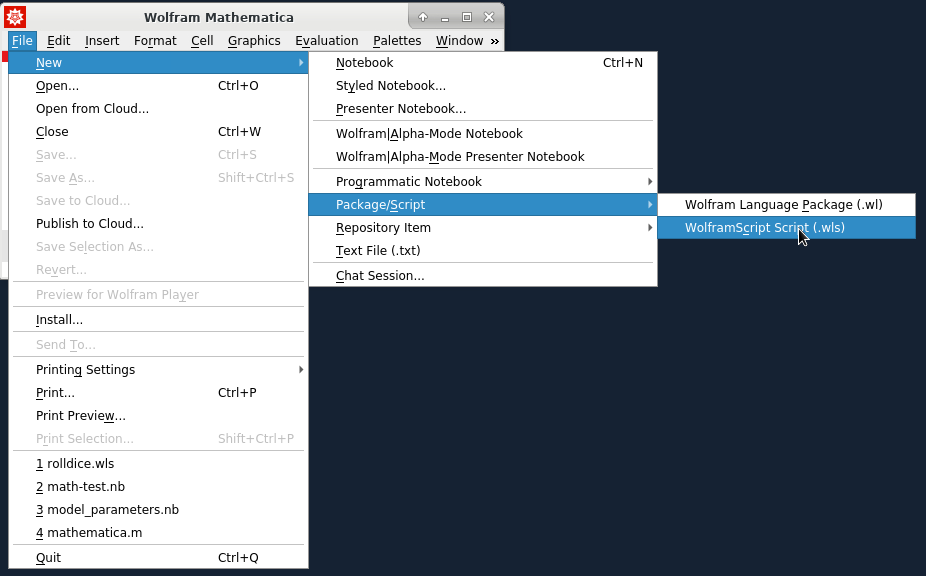
You may see different suffixes for Mathematica files, such as ".nb", ".m" and ".wl". The ".nb" file is the Mathematica notebook, and you can do the calculation in the notebook interactively through the GUI. If you write the code involving the packages or want to run on the cluster, then you may use the Wolfram Language Package format with the suffix ".wl". The ".m" is the old way (before version 10.0) of saving package files. To convert a notebook file to the ".wl" package file, the preferred way is open a new ".wl" file and copy the code from the notebook, then save it as the ".wl" file. Note: In the ".wl" file, you can use the Print to produce an output from the code. If the code does not explicitly print the results, the value of experession is not returned by default.
For example, suppose you have the code '"math-test.wl" as the following:
(* ::Package:: *)
x=7
3x
Print[RandomInteger[{1,6},2]]
You can evaluate the code which only prints the last expression since it has the Print statement,
wolframscript -file math-test.wl
Also, you can evaluate the code and print each output with
wolframscript -noprompt < math-test.wl
To submit Mathematica jobs to compute nodes, the Mathematica commands to be executed must be contained in the script. As an example, we will submit the previous code "math-test.wl" to the cluster. This job script submits the "math-test.wl" to compute node:
#!/bin/bash
#SBATCH --output=mathematica.o%j
#SBATCH --job-name=mathematica # create a short name for your job
#SBATCH --nodes=1 # node count
#SBATCH --ntasks=1 # total number of tasks across all nodes
#SBATCH --cpus-per-task=1 # cpu-cores per task (>1 if multi-threaded tasks)
#SBATCH --mem-per-cpu=4G # memory per cpu-core
#SBATCH --time=00:05:00 # total run time limit (HH:MM:SS)
module purge
module load Mathematicawolframscript -noprompt < math-test.wl
Wolfram Language can be used as the scripting for shell scripts. The Wolfram Language scripts should start with "#!/usr/bin/env wolframscript". For example, let's generate a random number between 0 and 1. First, create the script file:
then edit the Wolfram Language code and save the file:
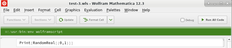
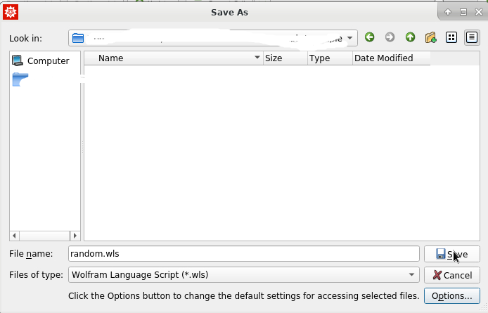
You can use the text editor to open the script "random.wls" :
#!/usr/bin/env wolframscript
(* ::Package:: *)Print[RandomReal[{0,1}]]
Set the script permission to make it executable and run the script:
chmod +x random.wls
./random.wls
The output will be the pseudorandom number between 0 and 1, for example, 0.9158465157932778.
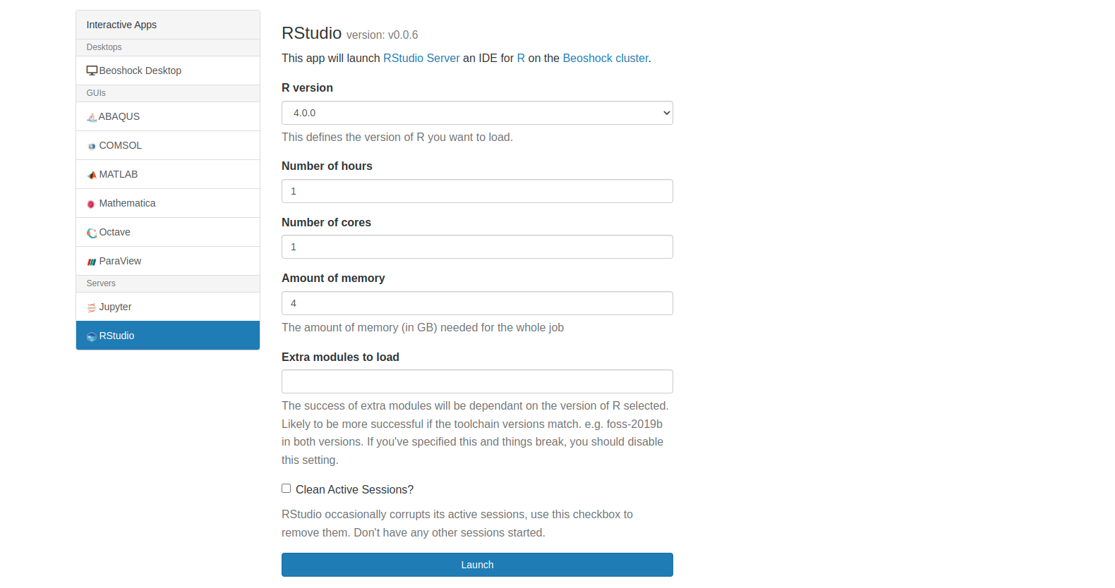
Using R on BeoShock
RStudio is available through Open Ondemand web portal. To connect to Open Ondemad, browse to ondemand.hpc.wichita.edu. Click on "Interactive Apps" and then "RStudio" to begin a session. You can set the allocation resources through "Number of cores", "Number of hours", and "Amount of memory".
After connect to the BeoShock cluster, load the R module and start R interactively:
module load R/4.1.0-foss-2021a
R
Then you can install the package using:
install.package("PACKAGENAME")
You can check the library by:
library("PACKAGENAME")
There are some packages available in the module environment, for example, rgdal package. If you want to use the rgdal package, type the following:
module purge
module load rgdal/1.5-23-foss-2021a-R-4.1.0
When you are doing production runs that need more computation power than a head node, it is advantageous to submit jobs to HPC. Once you have the R code saved in the ".R" file (i.e., test.R), you can use the R command in the job script. Here is the minimal example for a bash script:
#!/bin/bash
#SBATCH --mem-per-cpu=4G
#SBATCH --time=0-00:10:00# This starts R and loads the file test.R
module purge
module load R
R --no-save -q < test.R #--no-save prevent the saving of the workspace
QGIS
QGIS, is a free and open-source geographic information system (GIS) software application that allows users to view, edit, and analyze geospatial data. QGIS supports a wide range of data formats and provides tools for data visualization, spatial analysis, and map creation. It can be used for a variety of applications, including environmental monitoring, urban planning, and natural resource management. The documentation can be found at QGIS user guide.
For the first time to use the QGIS on Beoshock Desktop, you will need to set up the virtual environment in order to not give errors on startup.
-
Load the QGIS module by running the command:
module load QGIS -
Create a new Python virtual environment in the directory
~/virtualenvs/qgisby running the command:mkdir ~/virtualenvs/qgisandvirtualenv ~/virtualenvs/qgis -
Activate the virtual environment by running the command:
source ~/virtualenvs/qgis/bin/activate -
Install the following dependencies by running the command:
pip install pyyaml owslib psycopg2 jinja2 pygments -
Run QGIS by running the command:
qgis
Then on the subsequent sessions for BeoShock Desktop, follow these steps to run QGIS:
-
Load the QGIS module by running the command:
module load QGIS -
Activate the virtual environment by running the command:
source ~/virtualenvs/qgis/bin/activate -
Run QGIS by running the command:
qgis